Describing Data and Testing Hypotheses

Core

Variable Types

A variable records a property that can differ between observations. Before calculating anything, ask what kind of variable was measured. A neat spreadsheet column can still be analysed wrongly if its labels, ordering or measurement scale are misunderstood.

Categorical variables place observations into groups. Nominal categories have no natural order, such as blood group or organism species. Binary variables have two categories, such as event or no event. Ordinal categories have a meaningful order but unequal or unknown spacing, such as mild, moderate and severe disease. Coding categories as 0, 1 and 2 does not turn those labels into continuous measurements or make their mean automatically meaningful.

Numerical variables express counts or measurements. Discrete variables take separate countable values, such as number of admissions. Continuous variables can, in principle, take any value within a range, such as height or serum sodium concentration. Rounding may make a continuous measurement look discrete, but its underlying scale remains continuous. The outcome variable usually drives the analysis: a categorical outcome suggests comparing proportions, whereas a continuous outcome suggests comparing a centre or modelling a numerical change.

Centre and Spread

A measure of centre answers where observations tend to lie. The mean uses every numerical value and is efficient for a roughly symmetric distribution, but it is pulled by extreme observations and long tails. The median is the middle ordered value and is more resistant to outliers and skew. The mode is the most frequent value or category; it can be useful for categorical data but may be absent or multiple in a numerical sample.

Centre without spread is incomplete. The range gives minimum to maximum and is dominated by two observations. The interquartile range spans the middle 50% and pairs naturally with the median for skewed data. Variance averages squared deviations from the mean, so its units are squared. The standard deviation is the square root of variance and returns to the original measurement units. It describes how observations vary around their sample mean; it does not describe uncertainty in the mean itself.

Summary choices should be declared from the distribution and question, not selected after seeing which looks favourable. For a symmetric single-peaked distribution, report mean and standard deviation. For a markedly skewed distribution or influential outliers, median and interquartile range often communicate the data more honestly. Important clinical thresholds and the raw shape may still deserve display even when a compact summary is appropriate.

Distributions

A distribution describes the pattern of values, not just its average. A normal distribution is symmetric and bell-shaped, with mean, median and mode aligned. Many biological measurements are approximately normal within a defined population, but normality is a model, not a rule. A larger sample does not force the observed data themselves to become normal.

Right-skewed data have a long upper tail, often because most observations are small but a few are very large. The mean is usually pulled above the median. Left skew reverses that direction. Outliers may be genuine biology, data error or a member of a different population; they should be checked and explained, not automatically deleted. Histograms, box plots and quantile displays reveal shape that a mean and standard deviation can hide.

Parametric methods make assumptions about a model, often about residuals or paired differences rather than every raw measurement. They can be robust to modest departures when samples are suitable. Non-parametric or rank-based methods make fewer distributional assumptions about the numerical scale, but they still have assumptions and do not simply test the same quantity with less power. The scientific question should remain explicit: are you comparing means, distributions, ranks, proportions or an association?

Samples and Standard Error

A sample is used to estimate a feature of a larger target population. If repeated random samples were taken, their sample means would differ. The distribution of those possible means is the sampling distribution. Its spread is the standard error of the mean, which measures the precision of the estimated mean.

Standard deviation and standard error answer different questions. Standard deviation describes variation among individuals in the observed sample. Standard error describes how much an estimate would vary across repeated samples under the sampling model. Increasing sample size usually narrows standard error because more independent information stabilises the estimate. It does not remove systematic bias, repair poor measurement or make an unrepresentative sample representative.

The same logic applies beyond means: proportions, differences, ratios and regression coefficients have sampling distributions and standard errors. Independence matters. Repeated observations from one person, paired measurements and clustered participants do not contribute information as if every row came from a different independent individual.

Hypotheses, Confidence Intervals and P-values

The null hypothesis states a reference claim, often no difference or no association. The alternative hypothesis states the effect or association under consideration. A statistical test asks how compatible the observed data are with the null model and its assumptions.

A p-value is the probability, assuming the null hypothesis and analysis model are true, of obtaining data at least as incompatible with that null as the observed data. It is not the probability that the null hypothesis is true. It does not measure effect size, clinical importance, study quality or the probability that a result will replicate. A small p-value can accompany a trivial effect in a large study; an important effect can have a large p-value when data are imprecise.

A confidence interval combines an estimate with its precision. A narrow interval indicates greater precision than a wide interval on the same scale. In frequentist terms, a 95% confidence-interval procedure would contain the true parameter in 95% of repeated samples generated under its assumptions. For one observed dataset, use the interval as a range of effect sizes reasonably compatible with the data and model, while remembering that bias and model error are not captured by width alone.

The null value depends on the measure: zero for a difference, and one for a ratio. If a conventional 95% interval excludes its null, the corresponding two-sided test is generally below 0.05 when the same model is used. That relationship should not replace interpretation of magnitude and precision.

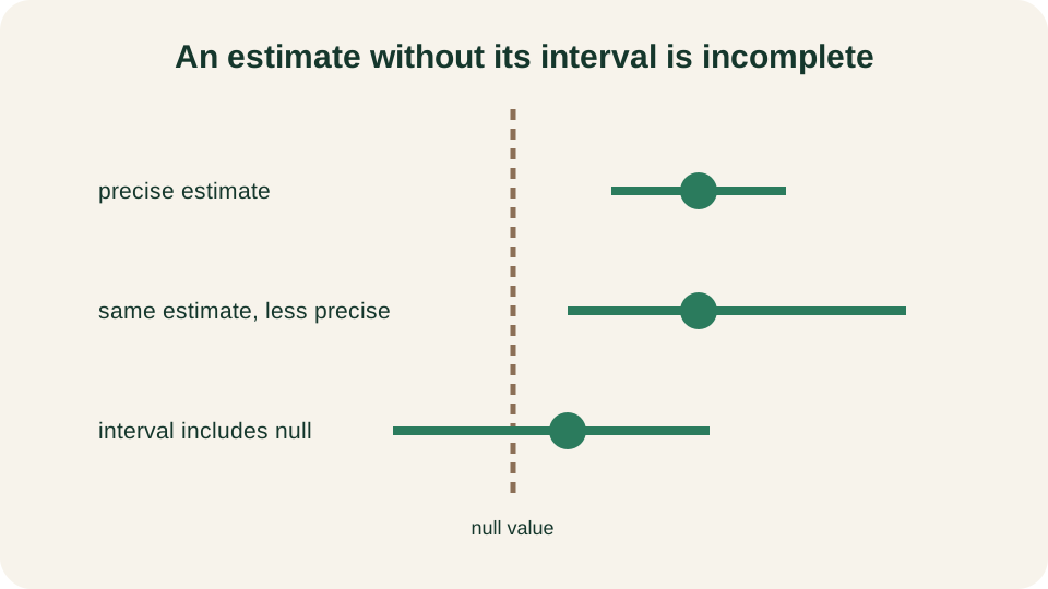
The point estimate gives magnitude; interval width gives precision; inclusion of the null addresses compatibility with no effect.

SimpleMed original educational diagram

Errors and Power

A type I error is rejecting a true null hypothesis, a false-positive conclusion. The prespecified significance level, alpha, controls its long-run probability for a valid test. A type II error is failing to reject a false null hypothesis, a false-negative conclusion. Beta denotes that probability for a specified true effect and design.

Power is one minus beta: the probability that the planned analysis detects a specified effect when it truly exists. Power increases with larger sample size, larger true effect, lower variability, more efficient measurement and, all else equal, a less stringent alpha. Raising alpha to gain power also increases type I error, so it is not a free improvement. Sample-size planning requires an effect worth detecting, anticipated variability or event rate, alpha, target power and allowance for loss or unusable data.

Failure to reject the null is not proof of equivalence. It may reflect a genuinely small effect, wide uncertainty, few events, high variability or poor measurement. Equivalence and non-inferiority questions need designs and margins chosen for those aims rather than retrospective claims from a non-significant superiority test.

Test-choice Tree

Choose a test by moving from question to data structure. First identify the outcome variable. For a categorical outcome, compare proportions using a chi-squared family test when expected counts are adequate, or an exact method when sparse counts make approximation unreliable. For a continuous outcome, decide whether the analysis concerns two groups, more than two groups, or a relationship across values.

Next ask whether observations are independent or paired. Measurements before and after treatment in the same person are paired. Matched participants and repeated measures also carry dependence. A two-sample t-test is a common parametric comparison of independent means; a paired t-test analyses within-pair differences. With more than two independent groups, analysis of variance is the corresponding parametric family. If the target is ordinal or assumptions for mean-based methods are unsuitable, rank-based families include Mann-Whitney for two independent groups, Wilcoxon signed-rank for paired data and Kruskal-Wallis for more than two independent groups.

Named tests are not interchangeable buttons. Check independence, outcome scale, group number, pairing, distributional model and whether the test targets the scientific estimand. Multiple comparisons, clustering and repeated measurements may require methods beyond this compact tree.

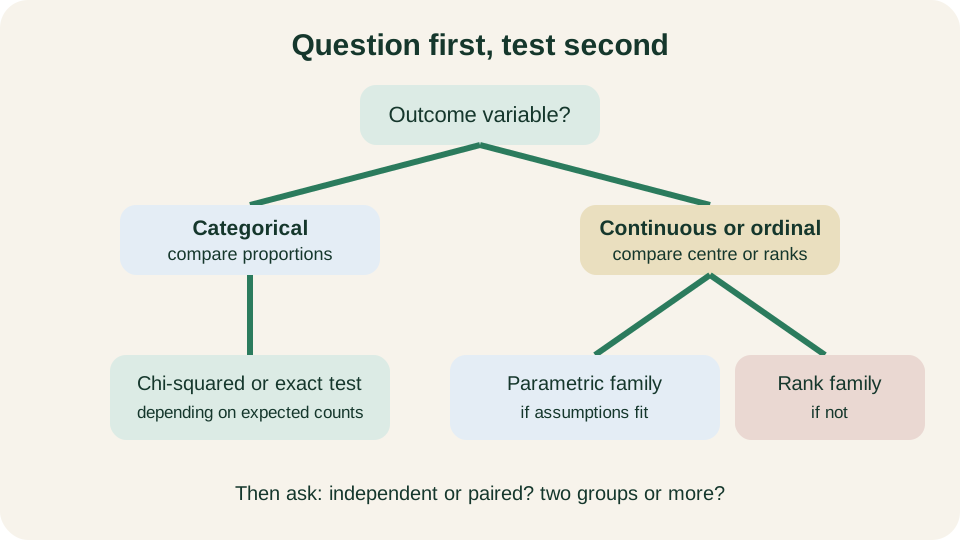
Start with the outcome and question, then narrow by groups, pairing, expected counts and model assumptions.

SimpleMed original educational diagram

Likelihood Ratios and ROC Curves

Likelihood ratios extend diagnostic-test reasoning by showing how strongly a result changes odds. The positive likelihood ratio compares the probability of a positive result in disease with that in no disease. The negative likelihood ratio compares the probability of a negative result in disease with that in no disease. A likelihood ratio of one does not change odds; larger positive ratios and smaller negative ratios produce stronger shifts. Pre-test odds multiplied by the relevant likelihood ratio give post-test odds.

A receiver operating characteristic, or ROC, curve plots sensitivity against one minus specificity as a continuous test threshold changes. Moving the threshold trades false positives against false negatives. The area under the curve summarises discrimination: the ability to rank a randomly selected case above a randomly selected non-case. It does not prove calibration, clinical usefulness, causal value or a universally best threshold.

Threshold choice depends on consequences and context, not geometry alone. Detailed sensitivity, specificity, predictive values and screening-programme criteria remain in Beliefs of the Public. Trial design and bias remain in Epidemiological Studies. Here the aim is disciplined interpretation: match summary to variable, test to question and conclusion to uncertainty.

Reviewed by: Dr. Marcus Judge

Quiz

Preview the Describing Data and Testing Hypotheses quiz